Python Plotting 1. Plotting the Monthly AverageTemperature from Daily Data.

Prerequisite:

conda environment with python3 iris library

Let's start off with basic plotting of Temperature data using the python library - Iris 2.2.0 (Refer previous blog on iris installation details)

Data Source:

Link: https://cds.climate.copernicus.eu/#!/home (ERA5-Land hourly data from 2001 to present )

European Centre for Medium Range Weather Forcasting (ECMWF) provides reanalysis and forecast dataset at surface as well as pressure levels of different meteorological variables and atmospheric compositions. Also, the dataset are freely available.

User just have to register and and then login to get access to the dataset. More information about the data is available on https://cds.climate.copernicus.eu/cdsapp#!/search?type=dataset

Temporal resolution : August 2018 (Daily data)

Now, Lets try to visualise what was the Average Temperature.

The python code for exploring and visualising data is below falong with the discription:

> cd /folder/where/met/file/is/downloaded

#% /usr/bin/env python
from six.moves import filter, input, map, range, zip
import numpy as np
import cartopy.crs as ccrs
from cartopy.mpl.gridliner import LONGITUDE_FORMATTER, LATITUDE_FORMATTER
import matplotlib.pyplot as plt
import matplotlib.cm as mpl_cm
import matplotlib.colors as colors
import iris.plot as iplt
import iris.quickplot as qplt
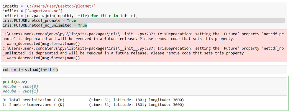
import os, sys   ## avoid the underlines...:)

all the above modules are to be imported or called for our analysis. Most of them are iris automatically downloaded/installed while downloading/installing iris and few are inbuilt but there are few that might need to be installed.  

inpath1 = 'C:/Users/user/Desktop/plotmet/' ## path where the met file is present

infile1 = ['August2018.nc'] ###file name###
infile1 = [os.path.join(inpath1, ifile) for ifile in infile1]
 ###os,sys tools to connect file name and file path#####
iris.FUTURE.netcdf_promote = True ####read netcdf (.nc) file in iris###
iris.FUTURE.netcdf_no_unlimited = True ####read netcdf(.nc)file in iris###

cube = iris.load(infile1)
###loading the August2018.nc file in iris cube###
###The top level object in Iris is called a cube. A cube contains data and ####metadata about a phenomenon. Here our downloaded met file is our cube  

print(cube)

The cube represents 2m temperature and total precipitation.There are 4 data dimensions, and the data has a shape of (31, 1801, 3600)The 3 data dimensions are mapped to the time, grid_latitude, grid_longitude coordinates respectively

##Creating Temperature and precipitation cube seperately
ncube = cube[0] # Temp
dcube = cube[1] # Precipitation

####Lets plot Temperature First######
#########################Applying Lat/Long Constraint###########
latitude_name = 'latitude'
longitude_name = 'longitude'
constraintDict = {latitude_name: lambda lat: 10 <= lat < 35, 
                 longitude_name: lambda lon: 52 <= lon <= 90}
constraint = iris.Constraint(**constraintDict)
### Defining regional constraint around Indian subcontinent###

#####subsetting the cubes over the regional constraints##### 

ncube1 = ncube.extract(constraint)
dcube1 = dcube.extract(constraint)

print(ncube1)

Latitude/Longitude shape is now reduced

ncube2 = ncube1.collapsed('time', iris.analysis.SUM)
dcube2 = dcube1.collapsed('time', iris.analysis.MEAN)
###From the daily data, we intend to find the monthly mean of temperature ##and total precipitaion

### lets see we have collapsed the time by averaging (incase of temp) and 
#### adding up incase of Precipitation
## Now we should have a 2-D cube with latitude and longitude coordinates 

print(ncube2)
print(dcube2)

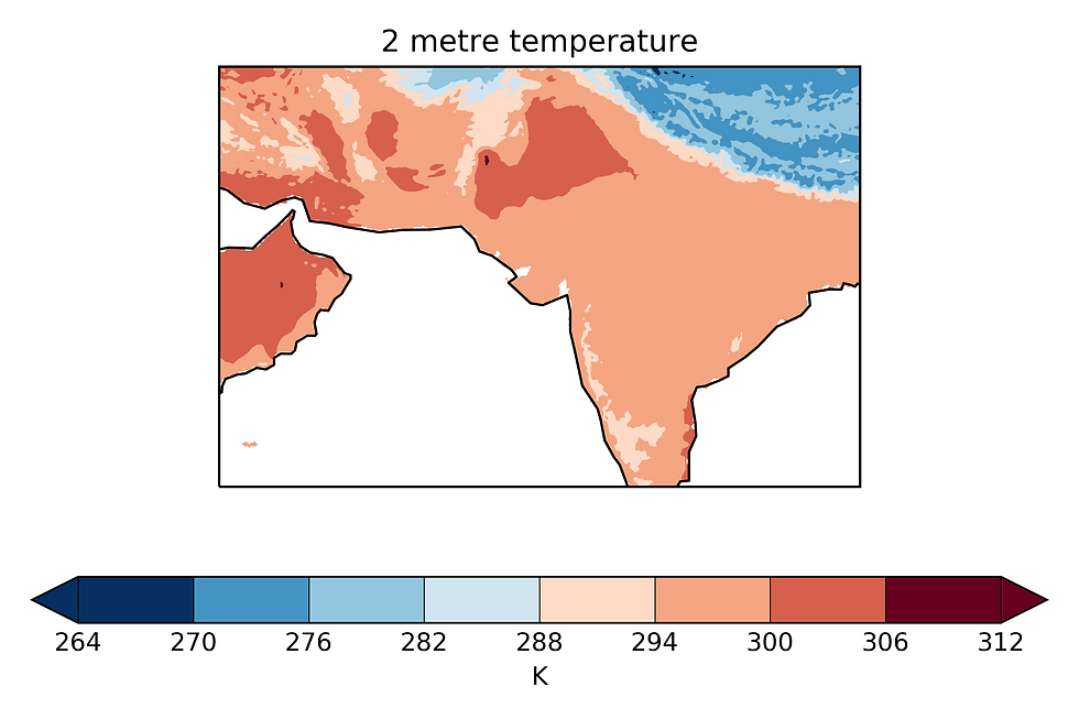
#####Lets plot######
brewer_cmap = mpl_cm.get_cmap('brewer_RdBu_11')
qplt.contourf(dcube2,  cmap = brewer_cmap, extend = 'both')
plt.gca().coastlines()
plt.tight_layout()
plt.savefig('August_Mean_Temperature', dpi = 500)
plt.show()

Temperature Plot